Chain Home and the Cavity Magnetron

A magnetron is a diode that can be made to oscillate.

This sounds impossible. A diode is a simple component with a single function - it lets current flow though it in one direction, but not in the other. But an oscillator is a complicated electronic circuit carefully designed to supply energy at a single frequency. An oscillating diode seems as unlikely as an oven that doesn't get hot, yet both are quite common. There's a magnetron inside every microwave oven, oscillating efficiently at ultra-high frequency and emitting nearly a kilowatt of energy that bounces around inside the oven and heats up the food.

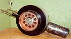
A cavity magnetron like the one shown on the left played a crucial role in radar systems in the early 1940s. It's small enough to fit in your pocket - the black metal disk is only 3" (7.5 cm) in diameter. The magnetron in your kitchen microwave oven was designed 60 years later, and looks nothing like this!

But before I describe how the device works, I need to explain why it was important, and that involves a brief look at the UK's wartime Chain Home radar defence system and how it came to be built.

In the early 1930s there was no such thing as radar, and it was generally agreed that "the bomber would always get through". There was some wild talk about Death Rays though, and so the Director of Scientific Research (DSR) for the Air Ministry asked the Superintendent of the Radio Research Department of the National Physical Laboratory at Slough to let him know if such a gadget could be built. The Superintendent - Robert Watson Watt - asked A.F. Wilkins, one of his Scientific Ofiicers, to do the sums. Wilkins duly reported that, if an aircraft could be irradiated from 600m for 10 minutes at a power level of 5,000 megawatts, the pilot's brain would indeed begin to boil.

Watson Watt thought that this power level was too low (not that it would have been remotely possible to achieve it) because the aircraft's metal skin would probably stop most of the energy from getting through. On the other hand, if the metal skin reflected some energy, it might just be possible to detect the reflections, and he did a few sums of his own to find out. It looked as though the idea should work. But the DSR's boss - Air Marshal Sir Hugh Dowding - didn't trust scientists, or their calculations, and demanded a proper test with a real aeroplane.

Detection of aircraft using radio

So on a freezing cold day in February 1935, Wilkins set off in a van from Slough, heading for Daventry. His mission was to demonstrate that it really was possible to detect an aircraft flying close to the big BBC transmitter there. Daventry was chosen because Wilkins had already measured the radiation pattern of its aerial and could make an educated guess about where the experiment was likely to give positive results.

The idea was to erect a couple of aerials 100 feet apart in a field five miles from the transmitter and connect them to a dual-channel receiver. Both receiver outputs would be connected to a CRT. By carefully adjusting the phase of one receiver input relative to the other, it should be possible to null out the ground wave, leaving a motionless spot in the centre of the CRT. But an aircraft moving nearby should reflect different levels of signal to each receiver, which should cause the spot to move.

Wilkins and his driver, Dyer, put up the aerials, and went off to find a hotel for the night. They returned after dinner to set up the receiver. It was dark by then, and there was no light in the van, so Dyer patiently struck match after match. Wilkins worked as quickly as he could, and shortly after midnight the system seemed to be functioning. They disconnected the aerials and got back in the van. It wouldn't move - it was frozen to the ground. Fortunately, they had a spade in the back and could dig themselves out. After a few hours sleep, they were back on site well before Mr. Watson Watt and the man from the Air Ministry arrived in the morning, and everything still worked.

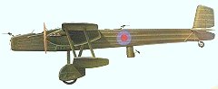
It had been arranged with the RAF that a Heyford bomber would fly over the BBC masts towards the van. Unfortunately, the pilot flew east instead of south-east, and although the observers on the ground could hear the aircraft, the spot on the CRT didn't move. Subsequent passes were more successful, though, and when the bomber flew nearly overhead, the spot grew into a line. The idea clearly worked. It really was possible to detect the tiny amounts of radio energy reflected from an aircraft.

The idea of radar

Using radio to detect that there was an aircraft out there somewhere was interesting, but not very useful. How could you work out where it was? And its altitude? And which way it was going? And whether it was alone in the sky? These questions needed answers before anyone could think about designing a system to exploit the idea.

Watson Watt already knew that it was possible to transmit pulses of energy and see their echoes (from the ionosphere) on a CRT connected to a sensitive receiver. Given a sufficiently powerful pulse, and a sufficiently sensitive receiver, he thought it should be possible to see aircraft as far away as 50 miles. Their altitude could be assessed by comparing the signals from receiving aerials mounted at different heights, and their bearing found from the relative signal strengths seen by several widely separated receiving stations.

Much experimental work needed to be done, and a suitable site was found at Orfordness, off the Suffolk coast. The radio industry knew how to make equipment that worked well at 6 MHz - the state of the art, at that time - so with a suitable aerial hung from a couple of 60 foot towers and the original pulse transmitter transported from Slough, Watson Watt and his small team began to explore how a workable radar system might be built.

The pulse length was shortened from 200 μS to 30 μS in order to reduce the minimum range at which reflections could be seen on the CRT, and the frequency was raised from 6 MHz to 11 MHz when this was found to decrease the receiver noise level. By July of 1935 the equipment was detecting aircraft 50 miles away.

Orfordness had proved that radar could be made to work, and now the team needed to grow. More space was required - for laboratories, bigger and better aerials, and above all, for more people. A better site was quickly identified at Bawdsey Manor, ten miles down the coast, and development was transferred there in 1936.

Early in 1937 specifications were being written - the transmitter must deliver at least 200 kW of pulse power, and 50 μV at the receiver input must produce a trace deflection of at least 1" - whilst work had already begun on constructing the first five CH sites. By the outbreak of war in September 1939 there were 19 operational CH stations, together with the plotting rooms and other infrastructure that put the information they collected into the hands of those who needed it.

Chain Home

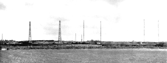
A photograph of a Chain Home station shows a few big towers in a field, but gives no clue as to what the towers were for. In fact, there were two sets of towers - one for transmitting, and the other for receiving.

The two tall transmitter towers (on the left) supported a curtain of end-fed horizontal dipoles, as shown in the diagram below.

Transmitting

The station was designed to transmit on one of four possible frequencies (to counter expected jamming attacks by the enemy), so three transmitter towers were needed for the four sets of dipoles.

From the length of the half-wave dipole it's straightforward to work out what frequency was used. Since half a wavelength was 18 feet (5.5m), a wavelength was 11m, which corresponds to a frequency of 27 MHz. In fact, most sources say that the frequency was 20-30 MHz. Today's mobile phones use frequencies a hundred times higher than this, but in the late 1930s it was not a simple matter to generate 250 kW at 30 MHz, nor to design a suitable receiver.

The task facing the designer of an aerial system is to arrange the structure so that as much as possible of the radiated energy goes in the right direction. A simple horizontal dipole by itself won't do - it radiates in all directions (except along its axis). The CH transmitter aerial array included a curtain of reflectors hung on the landward side to redirect this energy outwards, across the sea, to where it was useful.

The main problem in controlling the azimuth of the radiation (that is, the angle from the horizontal) is that the ground acts as a mirror, so it's practically impossible to send the energy out horizontally. The best solution is to keep the ground as far away as possible.

But some energy is always reflected from the ground, and unfortunately the reflection process adds 180 degrees of phase shift. This means that at some angle the reflected signal and the direct signal will cancel each other out. There is always an angle at which NO energy is transmitted.

The performance of an aerial is usually illustrated by means of its polar diagram, which shows how much energy (in relative terms) is radiated in each direction. The performance of the CH transmitter aerials looked something like the diagram on the right, with a null at about 5 degrees above the horizontal. With almost no energy being transmitted at 5 degrees, the system was effectively blind in this direction.

The blind spot was removed by adding a supplementary array, known as the gap filler, suspended underneath the main array. Its polar diagram was designed to radiate maximum energy at 5 degrees.

At 360 feet tall, the Chain Home transmitter towers were huge - just about the same height as St. Paul's Cathedral. This allowed their aerials to illuminate aircraft flying at 1,000 feet when they were still 40 miles away (and if the enemy aircraft were considerate enough to fly at 15,000 feet, they could be seen 150 miles away). But the transmitter array acted as a floodlight - it broadcast energy out to sea over a wide angle. This meant that a station had to be built every 20 miles or so along the coast, to give continuous overlapping coverage.

It also meant that the receiving antennas had to be quite sophisticated. A simple dipole antenna would detect the echo returning from an aircraft, but would give no sense of whereabouts the aircraft was.

Receiving

The receiving antenna towers were smaller and lighter. They were 240 feet high, and built of wood. In Echoes of war Sir Bernard Lovell explains that the receiving aerials consisted of two pairs of crossed dipoles at different heights. The aerials were used in pairs, as shown here, to determine both the bearing of the target aircraft and its height.

By comparing the relative strengths of the signals received by each of the crossed dipoles, using a goniometer - a sort of adjustable phase shifter - and finding a null point, it was possible to deduce the target's bearing. Then by comparing the relative outputs of the pairs of aerials at different heights (and correcting for the curvature of the earth) the height of the target could also be found.

It was time-consuming work, and needed concentration. Women turned out to be much better at it than men.

Effectiveness

Chain Home was built to give early warning of where bomber raids were coming from, and when, so that fighter squadrons could be scrambled to intercept them instead of simply patrolling in the hope of spotting the enemy. More effective use of fighters meant that fewer would be needed, and Government was acutely aware that there might not be enough.

The Battle of Britain was fought largely in daylight. Provided the fighters could be sent to the same area of sky as the bombers, they could see the enemy and engage. If the German High Command had understood the importance of Chain Home and seriously damaged it before concentrating its attack on the cities, things may have turned out very differently. As it was, German tactics switched from daylight raids to night bombing, where cities were still relatively easy to find, but bombers were not. The radar stations could still track the bombers, but the fighters sent to meet them could not see where they were.

Weaknesses

The CH system had two major weaknesses. It couldn't see low-flying aircraft until they were very close, and it was so huge and heavy that it couldn't be fitted to ships, let alone aircraft. Both these problems were a direct result of the choice of operating frequency.

Technology advanced quickly, and by 1939 a system developed by the Army CD group could deliver 25 kW pulses at 300 MHz (that is, at a wavelength of just 1.5m instead of CH's 11m.) A shorter wavelength meant a smaller and lighter aerial, which permitted more beam-shaping elements, which gave a narrower beam. On trial in July 1939 the system proved able to see aircraft flying at 500 feet 25 miles away. Watson Watt was impressed, and the Air Ministry ordered 24 copies of the equipment, which became known as Chain Home Low, to plug gaps in the radar coverage around the coast.

It also proved possible to fit a variant of the 300 MHz system into an aircraft. In 1939 a Fairy Battle was fitted with quarter-wave horizontal antennas on either side of the engine, and half-wave dipoles above and below the wing. The radar operator sat behind the pilot and directed him to the target via the intercom. Air Marshal Dowding was taken on a demonstration flight, and the system was shown to work. But its range was limited, and the unwanted reflections from the ground were a problem.

The way forward seemed to lie in shorter and shorter wavelengths - microwaves, in other words. The problem was that nobody in the world knew how to generate large amounts of power at microwave frequencies.

Early magnetrons

Magnetrons had been used as high-frequency oscillators in university physics laboratories since the early 1920s. This illustration is from Terman's Radio engineering (1937), and he says that magnetrons had been made to oscillate at frequencies as high as 30 GHz (that is, with a 1 cm wavelength), though even at lower frequencies their efficiency was a miserable 5 to 10%.

The device was relatively simple - a central cathode, with a split anode around it, and a magnetic field arranged to be in line with the cathode.

Terman helpfully includes a diagram showing how to make the valve oscillate. I suspect that the tuned circuit was usually a Lecher line - two short parallel lengths of metal with an adjustable bridging strap to change the frequency.

It's not obvious quite how this simple diode could be made to oscillate. But think about what's actually happening to the electrons in the space between the cathode and the anode.

The cathode is heated, which causes it to give off great clouds of electrons. They start to accelerate towards the positive anode, and in a normal diode valve they would smash into it at high speed like bugs into a windscreen. But the magnetron also includes a magnet (the clue's in the name, really) and electrons moving in a magnetic field do not travel in straight lines.

The left-hand rule shows what happens when a current flows in a magnetic field. The electrons are pushed in a direction at right angles both to their original direction and to the applied field. The diagram illustrates that the thumb and fingers are all at right angles to each other, like the corner of a box.

The magnetic field is trying to make the electrons travel in a circle around the cathode, whilst the electric field (between cathode and anode) is trying to make them move directly outwards towards the anode. The electrons are influenced by both fields, and are forced to take a curved path.

The actual path the electrons follow depends (of course) on the relative strengths of the magnetic and electric fields.

In a weak magnetic field (A & B), the path hardly deviates from a straight line. If the magnetic field is very strong (D), the electrons come zooming back to the cathode (and when they hit it, they liberate more electrons, which can quickly destroy the cathode!)

But if the magnetic field has the right strength (C) the electrons just graze the anode. A few stick to it, but many don't.

The end result is that a cloud of fast-moving electrons circulates in the space between the cathode and the anode.

Resonant cavities

Most oscillators are built around a tuned circuit - that is, a capacitor connected to an inductor. The capacitor has two parallel plates, allowing an electric field (that stores energy) to exist between them. The inductor is a coil of wire, allowing a magnetic field (that also stores energy) to exist inside it. Connecting C and L together lets energy flow between them. The values of C and L determine the resonant frequency of the tuned circuit.

Suppose the capacitor acquires a lump of energy from somewhere, so that it has somehow magically become charged. An electric field springs into existence between its plates. The plates are connected together by the inductor, so the electric field immediately begins to collapse, driving a current through the inductor. This current builds up a magnetic field inside the coil. Eventually, when the capacitor is fully discharged, the current stops. The magnetic field now has nothing to sustain it, and so it in turn begins to collapse. The energy it had stored reappears as a current flowing back into the capacitor, recharging it (but this time with the opposite polarity) and again establishing an electric field. When the magnetic field has dwindled to nothing, the current stops, and now all the energy is again stored in the capacitor's electric field. Energy is swapped back and forth between capacitor and inductor, like the water in a bathtub sloshing backwards and forwards from one end to the other. The smaller C and L are, the more quickly the energy sloshes to and fro.

The coil need not have lots of turns - one turn will do. And the single turn could take the form of a cylinder. And the whole tuned circuit (for that's what it is) could be milled out of a block of solid copper, if that turned out to be convenient.

The first cavity magnetron was made in just this way.

Some energy is lost when current flows through resistance, of course, so the active device driving the tuned circuit must regularly top up the energy level in the circuit. One way of looking at this is to think of the active device as a negative resistor of just the right value to cancel out the positive resistance in the circuit. Positive (that is, normal) resistance absorbs energy from the circuit. Negative resistance contributes energy to the circuit.

In a cavity magnetron, the energy losses are made up by energy taken from the circulating stream of electrons, and in rather a clever way.

The cavity magnetron

This photograph of a cavity magnetron shows what it looks like with the lid removed. It doesn't show that it must be placed within the jaws of a huge magnet in order to work. Like its glass predecessor, this magnetron consists of a central cathode, surrounded by an anode, sealed in a vacuum, and with an external magnetic field arranged to be in line with the cathode.

But this device includes a brilliant and simple innovation. Instead of splitting the anode and connecting it to an external tuned circuit, the inventors (Randall and Boot, at Birmingham University) used lots of identical resonant-cavity tuned circuits and put them inside the anode. This allows the circulating electron cloud to interact directly with the tuned circuits.

How a magnetron works

Suppose the magnetron is just starting up. Electrons begin to circulate around the cathode, going faster and faster. They travel at random speeds as the system sorts itself out and tries to settle into a stable state.

In other words, the electron current is noisy. It contains energy at all sorts of frequencies. And this noisy current is circulating close to a series of resonant cavities, which act as tuned circuits. If they see energy at frequencies near their resonant frequency, they seize it, and store it, swapping the energy between their electric and magnetic fields just like any other tuned circuit.

The energy oscillating around inside each cavity establishes its own field - the RF field - which itself now interacts with the circulating electron current.

Electrons passing though the RF field may give up some of their energy to it, slowing them down and leaving them to fall into the anode. Or they may gain energy from it, sending them back towards the cathode.

The effect is to thin out the cloud, causing the electrons to collect into bunches that rotate like the sails of a windmill (but not really).

Getting the RF energy out is not difficult. A pickup loop can be placed inside any of the cavities and coupled to an external waveguide to feed the load. In the lab, this was simply a string of car headlamp bulbs to absorb the 400 watts continuously delivered by the magnetron.

But a radar system uses short pulses of energy. The magnetron is switched on briefly, then switched off again. If it's only on for 1% of the time, the average power output of 400 watts means that the output power of the short pulse sent to the antenna is a hundred times bigger. 40 kW is a respectable amount of power, especially when delivered by something the size of a cigarette packet.

Suddenly, a laboratory curiosity had become the heart of next-generation radar. For the first time it was possible to generate significant amounts of microwave energy, and work began immediately on designing the new device into an airborne radar system to help the night-fighters. There were many problems to overcome, particularly with the brand-new type of aerial system that would be required. Instead of simple dipoles, a system operating at 10cm would need a scanning reflector dish, like a searchlight, mounted in the aircraft's nose. The problems were solved as they arose. Hand-built 10cm radar equipment (known as AI Mk.VII) began to be installed in Beaufighters early in 1942

Magnetron stability and efficiency

In the diagram just above (on the right) illustrating how the electron stream and the RF field interchange energy, I deliberately showed the adjacent RF fields as being 180 degrees out of phase with each other. It is quite possible that this may not happen by itself. In fact, it often didn't happen. There's no particular reason why it should.

The diagram on the left shows a magnetron with 8 cavities. When the device begins to oscillate, the signals in each cavity will have random phase differences from each other, and each will have managed to extract a different amount of energy from the electron current. The cavities are all coupled together via the rotating 'spokes', so the phase differences will jitter about until eventually some kind of steady state is reached, in which the RF wave propagating around the anode hits a resonance.

Resonance could occur if (for example) each cavity locked into a phase difference of 45 degrees from its neighbour, since 45 x 8 = 360 degrees. Or the phase difference might be 90 degrees, or 180 degrees. These are different modes of operation, and it turned out that the device delivers the most power in the so-called π mode, in which alternate cavities have 180 degrees phase difference. Once the magnetron has found a stable state it will stay there unless something disturbs it - like a sudden small change in supply voltage, or cathode current, or even arcing in a cavity. If that happens (and it's difficult to eliminate) the phase starts jumping again, and power output drops. It took another stroke of genius to see how to fix the problem.

Back at Birmingham University, the original magnetron had been developed to the point where it could deliver 70 kW, but its efficiency was a miserable 10%. Efforts to get more power out of it led to 'frequency jumping'. Then Prof. Sayers and Dr. Boot (yes, the same man, but now with his doctorate) tried linking every other slot together, with bits of copper wire. Every alternate 'capacitor' is now effectively connected in parallel. The instantaneous voltage across all the parallel 'capacitors' has to be the same. These tuned circuits are compelled to operate in phase with each other. Alternate cavities must then be 180 degrees out-of-phase with their neighbours, so the magnetron is forced to run in the π mode.

The result was almost magical. Efficiency jumped to 50%, and pulsed power output could be increased five-fold to 350 kW.

Magnetron in airborne radar

The AI Mk.VII (with the unstrapped magnetron) was designed as a quick-and-dirty fix to get microwave airborne radar into service as fast as possible. A hundred systems were built and installed in Beaufighters, and between them they destroyed over 100 enemy aircraft. Radar was still secret, so the night-fighter pilots' success was solemnly attributed to their exceptional night vision (and a persistent rumour began that night vision was improved by eating lots of carrots).

Its successor, the properly engineered AI. Mk.VIII, was ordered in quantity (2,000 systems) from two separate suppliers. It replaced the Mk.VII system in the Beaufighters as well as the earlier 1.5m Mk.IV and Mk.V fitted to Mosquitos.

The cavity magnetron first ran on the lab bench in Birmingham in February 1940. By that summer, the British and American governments had agreed on a deal whereby the British would share their military technology in exchange for American manufacturing expertise and capacity, producing equipment for British use. The first example of the resulting American centimetric radar, known as SCR-720, was test-flown in Britain in January 1943. It was ordered in large quantities as AI Mk.X, and was fitted to Mosquitos, then to Meteors, and later even to Vampires and Venoms.

Useful sources

My thanks to Doug Robb and everyone at the Air Defence Radar Museum at RAF Neatishead, near Norwich. You can easily spend a day there!

Books

• RDF1 Michael Bragg (Hawkhead, 2002)
  This comprehensive survey of radar development uses the official record to reconstruct what actually happened. It was privately published, and is well worth tracking down.
• The history of Air Intercept radar and the British nightfighter 1935-59 - Ian White (Pen & Sword, 2007)
• Radio engineering - Frederick Emmons Terman (McGraw-Hill, 1937)
• Admiralty handbook of Wireless Telegraphy Vol.II (HMSO, 1938)
• Microwave tube transmitters - L. Sivan (Kluwer, 1994)
• Echoes of war - Sir Bernard Lovell (Adam Hilger, 1991)
• Radar Days - E G Bowen (Adam Hilger, 1987)
• Boffin - R Hanbury Brown (Adam Hilger, 1991)
• Night intruder - Jeremy Howard-Williams (David & Charles, 1976)

Images

The photograph of the magnetron appears in the Radar Museum's guidebook. I suspect the photographs of the towers and the Battle may be Crown copyright. I drew the diagrams.

Other related pages on this site

• Engineering & physics index page >
• Energy storage in capacitors
• Energy storage in inductors