
This article shows that the attenuation characteristics of ordinary telephone cable can be flat to frequencies above 100 kHz.
Telephones operate in the frequency range 200 to 3400 Hz. There is no reason why the cables connecting them to the exchange should have a greater frequency range than this. Yet they do. ADSL is commonplace. How is that possible?
Telephone cable
| Weight/mile (lb) | Cu or Al | Dia (mm) | Res (Ω) | Loss @ 800Hz (dB) | Loss @ 1600Hz (dB) |
| 2½ | Cu | 0.32 | 434 | 2.06 | 2.8 |
| 4 | Cu | 0.4 | 275 | 1.31 | 2.2 |
| 6½ | Cu | 0.5 | 168 | 1.18 | 1.79 |
| ? | Al | 0.5 | 287 | 1.9 | 2.7 |
| 10 | Cu | 0.63 | 109 | 0.91 | 1.38 |
| ? | Al | 0.8 | 112 | 1.2 | 1.7 |
| 20 | Cu | 0.9 | 55 | 0.62 | 1.04 |
NB. These numbers assume a cable - that is, 2 wires. So a single conductor of 2½ lb/mile wire has a resistance of 217Ω per km.
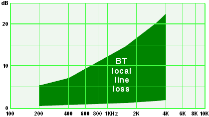
BT's document SIN351 says that BT lines are between 0 and 9km in length of 0.5mm copper with nominal characteristics of 168 Ω/km, 50 nF/km giving an attenuation of 1.7dB per km at 1600Hz.
However the document allows for considerable leeway. The expected range of losses is quoted as:
200 Hz: 5.1 to 0.4 dB; 400 Hz: 7.1 to 0.6 dB; 1600 Hz: 14.2 to 1.2 dB; 3200 Hz: 20.1 to 1.7 dB; 4000 Hz: 22.5 to 1.9 dB.
Wire tables list 24 AWG copper wire as having a diameter of 0.511 mm and a resistance of 84.2 Ω/km, so a pair would be 168 Ω/km, as SIN351 says.
Simple model
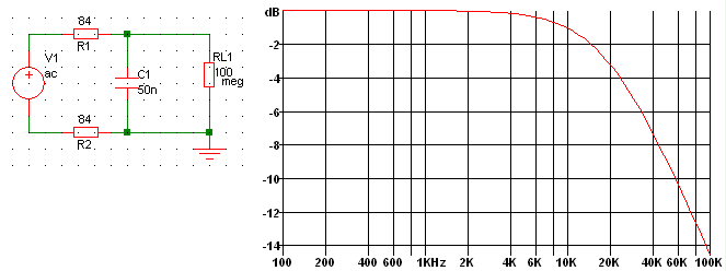
The simplest possible model of 1 km of "typical" local line cable could therefore be modelled like this ...
- and would display a simple first-order frequency response.
The model could (and should) be made more representative of a real cable.
More sections?
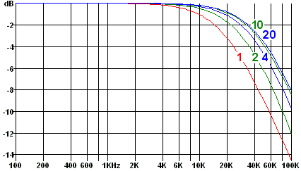
For example, the single 1 km section could be replaced by two or more shorter sections.
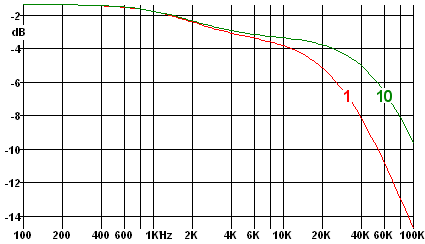
The graph on the left shows simulated results as the number of sections is increased as far as 20 (with R and C values adjusted to give the correct totals, of course.) Reassuringly, the results for 10 and 20 sections are very similar, so it seems unnecessary to model the line as more than 10 sections.
Terminating the line
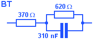
BT say in SIN351 that the cable should be terminated in a complex impedance that can be modelled as shown on the right.
Running the simulator with the line modelled as 1 section, and as 10 sections, shows that terminating the line with this impedance has introduced an extra loss of 3 dB between 2 kHz and 20 kHz.
Inductance of the wire

But this model has so far taken no account of line inductance. Each wire has an inductance of around 3 mH per kilometre (as I show here for example) and the resonant frequency of 3 mH and 50 nF is only 13 kHz. How much does inductance affect the results?
As the simulation shows, including the wires' inductance in the model makes a huge difference! The response is now substantially flat to about 250 kHz. (Above that frequency it drops like a stone, and is 250 dB down by 500 kHz.)
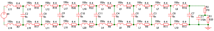
The 10-section model of 1 km used in the simulation
Real cables
The idea that ordinary telephone cable has a flat response out to 250 kHz seems extraordinary. I thought it was impossible. So I looked for some real data. I found an interesting article on the web:
"CABLE CHARACTERISTICS FOR FIELDBUS" by Stephen D. Anderson (Analog Services, Inc.)
in which he measured the characteristics of 15 representative cables. He found that their attenuation at 100 kHz was typically 7 dB.
However, his measurements were made with the cable pairs terminated in 95 Ω in series with 300 nF. Using this termination for my 10-section simulated line gave results very close to those he published, so it may be that this is not the optimum terminating impedance.